A/B testing is a common practice in web development. Two variants (A and B) of a page or product are presented to two randomized subsets of users. By comparing the responses to these pages, we can determine if one is better than the other.

At YourMechanic, we have built our own A/B testing platform, tailored to our needs and independent of third parties. In this post, we explore the statistics behind the platform. Other important topics, such as the randomization of users and assignment to buckets, in addition to the "product definition" of the platform, will be described in future articles.

Defining and measuring success

Suppose we want to explore a potential improvement for a page on our website. To measure this improvement, it is important to determine what we are trying to accomplish, and define proper goals. For instance, if we change the color of a button, do we want to increase the number of clicks, or are we trying to drive more purchases after visitors have clicked? In many instances, success is measured along several lines, and it is not uncommon to see a variant performing better for a goal and worse for another. In such instances, it is the role of the experimenter to weigh the different trade-offs.

To keep things reasonably simple, we will just assume that we are working with one goal in mind. We want to increase the rate of visitors who click on a button. We split our visitors 50/50 for each variant and end up with the following results:

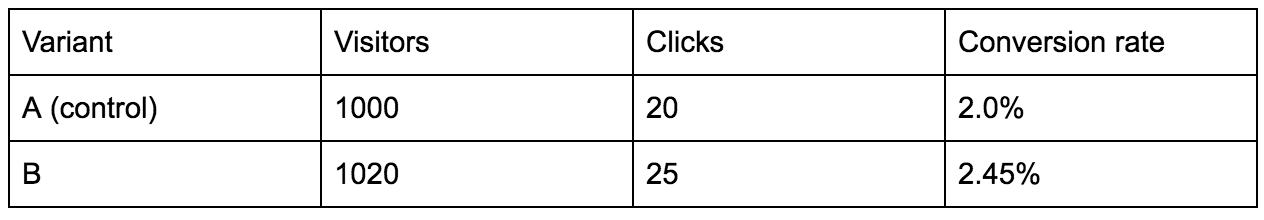
It is usually difficult to get a perfect split, but the counts of activations (unique visitors on the page where the test is performed) should be fairly close.

In this case, the control yields a lower conversion rate than the variant. However, this does not necessarily mean that B is better. How can we be certain that we have observed enough visitors? What if this result was only due to chance? We need some sort of measure of confidence to help us make a decision.

Bayesian approach

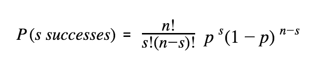
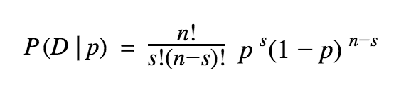
We can model the problem as a Bernoulli process: a person visits the website, flips a coin, and converts if the coin lands on the head. This is repeated many times, and each trial is independent and identically distributed. In other words, we get a sequence of n visitors landing on the page and among them s successfully convert. However, we do not know the parameter p (probability of converting). The probability to get s successes in n trials is:

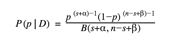
The parameter p is unknown, but we have data D in the form of the number of s successes out of n trials. Given this data, we would like to estimate a distribution on p. Using Bayes’ theorem:

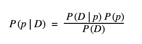
• P(p | D) is the posterior, it’s the distribution of p after we receive the data D
• P(p) is the prior, it’s the estimate of the probability of p before we receive the data D
• P(D | p) is the likelihood of observing D given the parameter p
• P(D) is the marginal likelihood, and does not depend on p

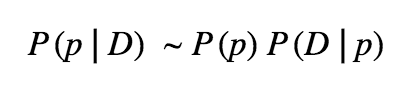
Therefore:

The likelihood is given by the same equation we saw above:

The common choice for a prior of the binomial distribution is the beta distribution (conjugate prior), with parameters α and β:

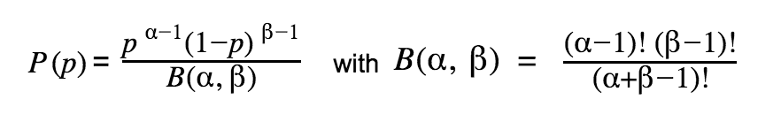
We can choose our prior based on historical data for conversion rates, or pick a simple uniform distribution Beta(1, 1). If we gather enough evidence the choice should not matter much in the end. With the simple uniform prior, we can write our posterior as:

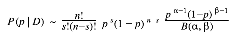
So, the posterior has the form:

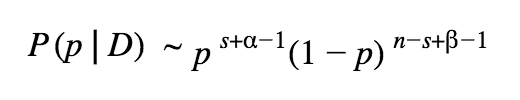
After normalization, the posterior is just a Beta distribution itself:

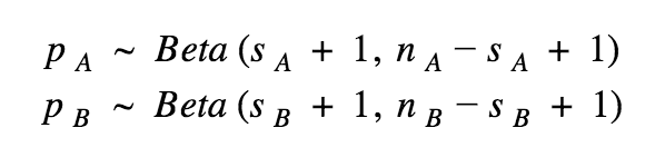
Assume we pick Beta(1, 1) as our prior, we can express the posteriors for the variations A and B as:

We want to know which version performs better, therefore we can look at P(p_A > p_B). What is the probability that p (conversion rate) is greater for A than for B? We can compute this probability by performing a direct integration of the the joint distribution, either numerically or computing it by hand, or we can use a Monte-Carlo method which is more brute force. We will use this method going forward.

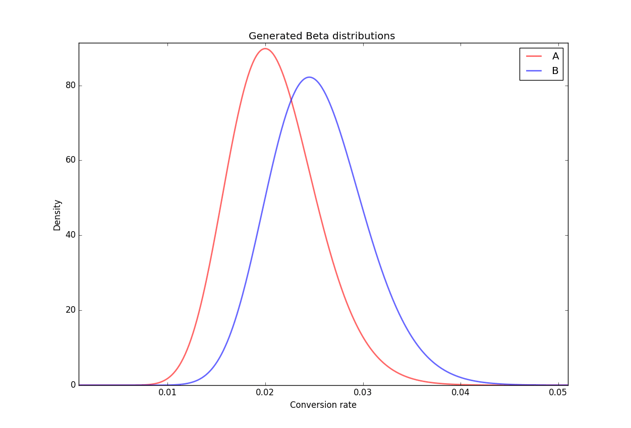
We generate the two beta distributions for A and B based on our counts of n and s, and then sample one point from each distribution: c_A and c_B, and we repeat this process for several iterations. We can compute an approximated lower bound for the number of samples required, but in most practical cases, 100,000 or 1 million simulations are enough and do not present computational issues for modern hardware.

We then count the number of simulations where c_A > c_B. If this is the case for C simulations, the probability P(p_A > p_B) is simply given by the ratio C/N. Now that we have the probability that the variation A is better than the variation B, how do we know when to stop the experiment?

In theory, we would like to wait for statistical significance, i.e. P(p_A > p_B) above a pre-fixed level chosen before the start of the experiment, typically 0.95 or 0.99 (or below 0.05 or 0.01 if B is better than A). Yet, we can run into some practical issues.

First, the probability may converge early above the threshold, before going back down. This can be seen when running a sufficient number of simulated A/A tests. To prevent making an early decision and face a type I error (false positive, i.e. conclude that there is a difference while it is not the case), we can enforce a condition that the test has to run for at least some period of time and have some 'sufficient' number of visitors before we end it, or we can use a better prior than Beta(1, 1) that would smooth out wider variations at the start of the experiment. Still, this is a dirty fix to prevent very early stopping of the test, but it is not a cure to type I error.

In addition, how long do we have to run a test before reaching significance? If the conversion rates between the variations are not very different, or if the traffic is low, we might need to wait a lot before reaching the desired P(p_A > p_B). We can compute an expected number of visitors needed to reach significance if current trends hold. In case our probability P(p_A > p_B) is still indecisive, we can decide to stop the test if the expected numbers of visitors required to reach significance is too great compared to what is reasonably feasible with our daily traffic.

How many visitors?

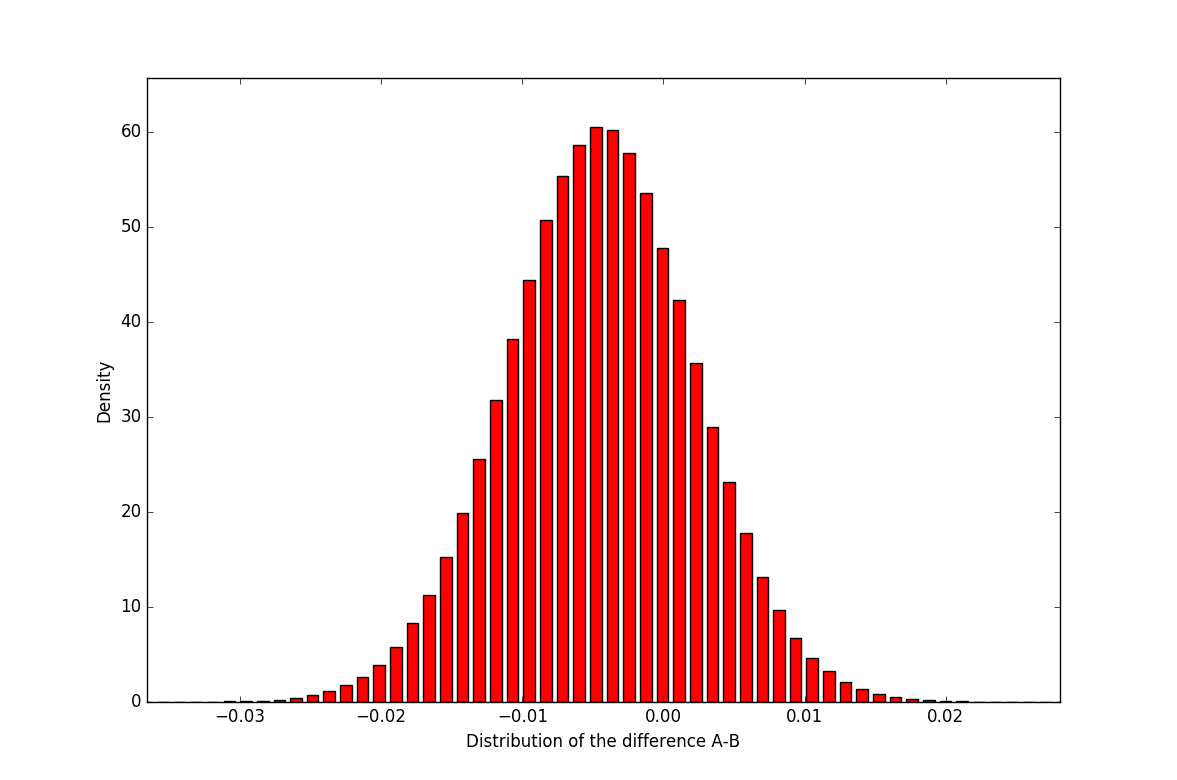
To determine how many visitors we need, we can compute the distribution of the difference between the two beta distributions representing the conversion rates for A and B. If we sample a large number of couple of points (below 10,000,000 points) from these distributions and compute their differences, we get the following distribution:

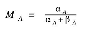
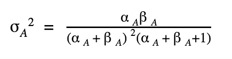
With α, β >> 1 and α ≃ β (which is usually the case with more than 1000 visitors and if the conversion rate is below 20-30%), we can locally approximate the two beta distributions with normal distributions N(M,σ).

The distribution of the difference is thus a Gaussian characterized by its mean and variance:

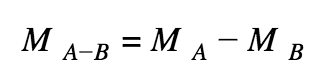
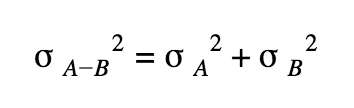
With (similarly for B):

Let’s assume that B is better than A.
How many visitors would we need so that P(p_A > p_B) < 0.01?
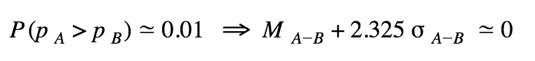
The probability P(p_A > p_B) is given by the area under the curve, to the right of 0.
We also know that if we integrate a normal distribution from infinity to the opposite tail up to ≃ M ± 2.325σ (depending on which way we are going) then we get an area under the curve of approximately 0.99.

Now, if we assume that the conversion rates for A and B stay the same, and continue using a prior of Beta(1,1) for simplification, we can compute an expected number of visitors to reach significance. Indeed:

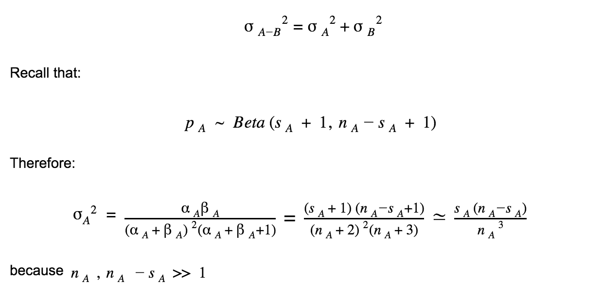
We assume a fair split between variations, thus n_A ≃ n_B ≃ N. Also, we assume that conversion rates stay constant, thus M_A = s_A/N and M_B = s_B/N. Finally:

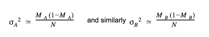
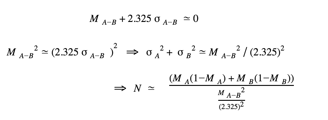
All we need are the values for M_A and M_B to compute N the approximate number of visitors per variation that we need in order to reach significance if the conversion rates remain constant. Of course they will probably not stay the same, so we will need to recompute this number from time to time. It is important to see this number just as an indication of an 'ETA' for the experiment to end.

Usually, if the experiment has been running for some time, and the expected number of visitors is very large (for instance, would require the experiment to run for many more months), it is likely that the experiment is unsuccessful and we have failed to prove that there is a significant difference between the two variations. After closer consideration, the experiment may be ended.

Recap

We have explored a simple way to compute the probability that a variation is better than another in an A/B test experiment. We have not touched upon more complex scenarios, and many improvements can be made on this base model, which, in addition, is certainly not the only possible approach (e.g. frequentist inference). For instance, what if we want to test more variations than just two (multivariate testing)? What if we want to compare purchase volumes instead of mere conversions? These will be topics for another day!

If you want to disrupt the auto repair industry, we are looking for software developers to join us and help us improve our tools and exciting core products!