Marketplaces by nature cater to two different customer sets - service providers and service consumers. A fundamental objective of any marketplace is to enable the service providers to get more work (i.e. be more “utilized”) and as a result, earn more, while at the same time providing the service at the earliest possible time to the service consumer. However, these are opposing forces. If a service provider is completely booked, the service consumer doesn’t have available times to choose from; if a service consumer has more times to choose from, it consequently means that the service providers are not fully booked. For optimal operation, the marketplace needs to find the equilibrium where the service providers are utilized the most possible, while service consumers have a reasonable number of available times to choose from.

At YourMechanic, we work with a nationwide network of partner mobile mechanics to help connect them with customers with car repair needs. The mechanic goes to the customer’s specified location to render the car repair services. In our case, the service provider is the mechanic and the service consumer is the car owner. While the following study was performed with respect to this ecosystem of mechanics and car owners, it can be applied to any corresponding eco-system where there is a similar service provider and consumer model.

Let’s start by first considering the ideal solution with respect to each side of the marketplace individually.

• For the car owners, the ideal solution is to let them see all the available time-slots so they can book the earliest available one or the one that works the best for their schedule. This is the scheme that we are using in our current scheduling system. This, however, is sub-optimal for the mechanics because they may now have consequent appointments at opposite ends of their service areas and end up spending large amounts of time in transit.

• For the mechanics, the ideal solution is to know the services at the beginning of the day so they can be optimized for maximum utilization as they can order the appointments to minimize time spent in transit. This is sub-optimal for the car owner as s/he doesn’t get to know the actual time of the appointment until the day before. It also limits the ability to book same-day appointments.

The ideal solution for the marketplace is somewhere in between, which provides certain degree of flexibility on both sides.

This blog will first propose the ideal solution to mechanics, in which we know all the jobs to be scheduled for the next day beforehand without any specific starting times. The solution prescribes the best route of appointments for each mechanic on the next day so that the mechanics can be utilized for the maximum possible hours. This “end-of-day” model provides us an upper bound on the utilization of mechanics.

Next, we consider a scenario in between the ideal scenarios of the car-owner side and the mechanic side. For example, we could ask a car owner to specify a preferred range of starting time of the job in a day and optimize the mechanics’ routes subject to the time-range selection; or we could ask a car owner to specify one or more mechanics s/he would like to work with, and optimize the starting time of the job among this pool of mechanics.

The following method demonstrates how the utilization could be improved compared to our current utilization.

The end-of-day model

The end-of-day optimization model is based on the assumption that we know all the jobs to be scheduled on the next day beforehand. We propose a Mixed Integer Program (MIP) that prescribes the optimal starting time and mechanic assigned to each job so that we can fit as many hours as possible to mechanics, subject to the constraints of mechanic availability, qualification and travel time. Each mechanic will be notified about his/her best route of appointments before the next day starts.

We partition our mechanics into several geographic regions (such as DMA regions, states) so that each mechanic’s service area is within a unique region. Therefore, we could use our model to optimally schedule mechanics in each region.

Now we are going to walk through the construction of our model.

Sets

We have three index sets to define the scope of the model: jobs, mechanics and time slots.

To use our past data to simulate the number of additional appointments that we can fit in a day using the end-of-day model compared to our current scheduling, we randomly select a set of jobs out of the quotes before the next day starts in addition to the booked appointments in current scheduling system.

Given a specified day and geographic region, the set of potential jobs that could be booked, J, is defined following the procedures described below:

• A = set of appointments that were booked to be completed on the specified day
• Q = set of quotes that a.) were quoted on the day before the specified day, b.) could start on the specified day, c.) did not convert to appointments on the quoted day, and d.) did not convert to an appointment on the specified day previously by the same user.
• w = maximum conversion rate of quotes on a day
• n = maximum number of quotes that could convert on a day; n:= ceiling(|Q| * w)
• Q' = set of converted quotes (i.e., booked as appointment); Q' = randomly selected n quotes from set Q
• J := A union Q'

Input parameters

Input parameters are the known data of our model, which define the coefficients in the constraints that describe the relationship between decision variables. Mechanic's time availability on the next day are known as a priori, in 15-minute time slots. Each job's location and duration (in minutes) are known as a priori. For each job, mechanics who serve the location of that job and have met various requirements to complete that job are considered as qualified mechanics for that job. We also need to define the rush hours and regular hours during the day and their corresponding travel speeds.

Decision variables

Decision variables are the unknowns of the model, which will be prescribed a value when we solve the problem to optimization. A binary variable can only take a value of either 0 or 1, while a continuous variable can take any real value in its specified range. The primary decision we need to prescribe is which mechanic is doing which job starting from which time slot. We also need several auxiliary decision variables to describe the usage of time slot per mechanic, the order of jobs assigned to each mechanic and the travel time in regular vs. rush hours.

Objective and constraints

The objective of our model is to maximize the utilization of mechanics (i.e., total minutes of jobs assigned to mechanics) on a specific day in a specific geographic region. The constraints we need to abide by are: 1) per job, there is at most one qualified mechanic assigned to perform it, 2) per mechanic, each of his/her available time slot can only be used by one job, and 3) there should be enough travel time between two adjacent jobs assigned to the same mechanic. Detailed explanation of each constraint will be discussed after we present our model.

(0) is the objective function, which maximizes the total scheduled duration of jobs that are assigned to mechanics.

(1)-(14’) are the constraints that define the solution space of decision variables.

(1) makes sure that for each job, at most one mechanic is assigned to do this appt.

(2) makes sure that if a job is assigned to a mechanic m to start at slot s, mechanic m must be available at slot s.

(3) makes sure that mechanic m must be available for the duration of job j if this job is assigned to mechanic m.

(4) makes sure that for each available slot s of mechanic m, at most one job could use this slot.

(4') makes sure that mechanic m must be qualified to do job j if the job is assigned to m.

(5) relates starting slot to the starting slot assignment.

(5') states that the ending slot of each job should not exceed the end of the work day.

Constraints (6)-(10’) define the rush hour indicators of the ending time slot of each job.

(6) and (6’) make sure that if the ending time slot of job j is no less than the starting time slot of morning rush hour, α_j must be 1. Here U is an upper bound on the number of time slots a job can have. We could use U = 96 here because there are at most 96 15-minute time slots in a day.

(7) and (7') make sure that if the ending time slot of job j is no greater than the ending time slot of morning rush hour, β_j must be 1.

Similarly, the pairs of constraints (8) and (8') / (9) and (9') relate the ending time slot of job j to the evening rush hours indicators.

(10) and (10') state that if the ending time slot of job j is either in the morning rush hours or evening rush hours, r_j must be 1.

(11) relates that the travel speed between jobs j₁ and j₂ to rush/regular-hour indicators.

(12) and (12') state that jobs j₁ and j₂ cannot be assigned to mechanic m adjacently if not both of jobs j₁ and j₂ are assigned to mechanic m.

(13) makes sure that there is at most one order of assignment of jobs j₁ and j₂, i.e., either j₁ starts before j₂, or j₂ starts before j₁.

(13') states that if both jobs j₁ and j₂ are assigned to mechanic m, one of v _{j1 j2 m} and v _{j2 j1 m} must be 1.

(14) and (14') state that if job j₁ starts before job j₂ , then the difference between their starting slots must be at least the duration (in terms of slots) of job j₁ and travel time between jobs j₁ and j₂.

(15) – (21) define the binary decision variable spaces.

Test run results

We run the end-of-day optimization model for a specific geographic region in a specific week. The working hours are defined as 7:00 am to 9:00 pm, in which the rush hours are defined as 7:00-10:00 am and 3:00-7:00 pm.

For each day, we randomly sample the set of quotes (i.e., Q) to obtain the set of converted quotes (i.e., Q’) 100 times to find an average improvement of utilization using our end-of-day model. On average, the utilization of mechanics is improved by 45%. The maximum improvement we archive in one day is more than doubling the current utilization. These results show that the optimization model helps fit in more appointments in a day without violating the availability, qualification and travel time requirements.

Procedure for customized time block selection

The end-of-day model is promising in improving mechanic utilization compared to the currently customer-centric scheduling, fitting in more jobs for the service providers and making them more content about their earnings. However, this is not going to make the customers happy because they have no choice over preferred time or mechanic, but have to wait until the beginning of the appointment day to be notified about the who and when their jobs would be performed. Therefore, we need to find a solution in-between. As we point out in the introduction, there are different ways to provide certain flexibilities to the customers.

In this section, we are going to explore the option of including customized time block selection, in which a time block is a number of consecutive time slots. For example, we could partition our working hours into 4-hour blocks, and ask each customer which time block s/he would like to start the job on the next day. Then we assign mechanics to jobs optimally each time a job is booked. Mechanics will be noticed about the scheduled orders of jobs before the appointment date.

Note that the mechanic and specific starting time assigned to a job could change as more and more jobs are added to the model, but the customer-specified starting time block of each job will not be violated. The model evolves to optimize the routes for the current set of booked jobs and leave us the capability to accommodate more incoming jobs. In other words, we are calling our end-of-day optimization model iteratively to add jobs one-by-one with additional constraint of customized time blocks.

Algorithm

Per day, per geographic region, we run several trials (K trials) to sample the quotes in set Q to obtain set Q'. In each trial, we iterate over jobs in set J (J = A union Q') to add customized time block selection into our model. After the set of potential jobs, J, is defined, we add jobs one-by-one to problem P in ascending order of quoted timestamps. Each customer can select an available time block to start their appointment on the next day.

Per trial, we could also run several times of the random time block selections so as to see the impact of time block selection sequence on utilization.

The algorithm is described below.

Obtain mechanic availability B_ms for m in M, s in S.

• For trial k in (0, K]:

  • Q'(k) = randomly selected n quotes from set Q
  • J(k) = A union Q'(k), sorted by ascending order of quoted/booked timestamps
  • Initialize the optimization problem P with all decision variables and objective function, but no constraints
  • JP = set of added jobs in the scheduling, JP = Null
  • B_ms (k) = matrix of mechanic availability after jobs are assigned, B_ms (k) = B _ms

  • For iteration i in [0,|A|+n):

    • for job i in J(k), obtain L_i, H_im, obtain D_j1i for each job j₁ in JP
    • generate a list of available time blocks for job i:
      • find a list of qualified mechanics with available time slots B_ms (k) for job i
      • find the overall available time slots for job i among all qualified mechanics
      • find the indices of available time blocks that job i can choose from
    • if there is no available time blocks:
      • add job i to the next day job list
    • else, add job i to problem P:
      • add constraint (1) for j = i
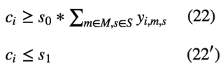
      • randomly select a time block that is available to job i, assuming the start and ending slots of selected block is s₀ and s₁, respectively.
      • add constraints (22) and (22') to problem P for the time block selection
      • 
      • add constraints (2) - (14') associated with job i to problem P, by replacing (1) j as i, (2) j₁ in J as j₁ in JP, and (3) j₂ as i
      • optimize problem P
      • update JP = JP union {i}
      • if sum{m in M, s in S}y_jms = 1, change constraint (1) to equality for j = i. This step makes sure that job i is always assigned to some mechanic, otherwise add job i to the next day job list
      • update B_ms (k) using the following equation
      • 

Note that the availability of mechanics is changing each time we schedule a job, so a later job may not have any available time block to choose from given the assignment of previous booked jobs on this specified day. In such situation, we have to schedule the later job to a later day.

Another result of adding a new job to problem P is that the new job is not assigned to any mechanic in the optimal solution, which means that even though there are available time blocks for the customer to choose from on the specified day, there is not enough travel time for mechanics to transit between previously scheduled jobs and this new job. In such situation, we have to schedule the new job to a later day. When we have to schedule jobs to a later day, we could put these jobs to the set J of the next appointment day and apply the same algorithm for the next appointment day.

Test run results

We take the same geographic region and pick a specific day to test our customized time block selection procedure. This experiment is to see how the sequence of time-block selection is affecting the utilization. On this day, we construct the set of potential set of jobs, J (J = Q’ union A), using the the first 50 trials of the random samples Q’, and run 10 random time-block-selection simulations in each trial. We partition our working hours to 4-hour time blocks.

The average utilization dropped 1.4 percentage points compared to the end-of-day model, which is not very significant. We can still preserve 90% of the improvement that we have achieved in the end-of-day optimization. Therefore, this in-between solution is balancing the needs between the service providers and customers, and still shows great potential to improve the utilization of our current scheduling system.

Conclusions and future research

The proposed model is a very flexible MIP that could be applied in different applications of on-demand, point-to-point services, such as scheduling technicians, drivers and specialists, to deliver a certain set of services. We consider many realistic business requirements of scheduling, such as availability and qualification of service-providers, different travel speeds in rush hours and regular hours between jobs, and time window restrictions. Traditional vehicle routing problems with time windows cannot deal with the constraints of qualifications of doing certain jobs without augmenting the network of enumerated assignment routes to each service provider. Generalized assignment problem is flexible to deal with qualification constraints, but not prescribing orders between assigned jobs. Compared to existing scheduling models in literature, our model incorporates comprehensive business requirements for job assignments as well as prescribes the optimal routes for each service provider. For different applications, the length of a time-block and the frequency of running the procedure can be customized.

Currently, we are using the PuLP package in Python with Coin-OR CBC open-source solver to model and solve the problems. In the future, we could design some heuristics to improve the run-time with reasonable gap from the optimal solution.